by Arjun Chandran

 

Neural networks are often associated with some of the remarkable things that artificial intelligence (AI) is capable of doing today, ranging from face and voice recognition to tumor detection. But how do neural networks actually work? Modeled after the brain’s biological networks, neural networks are a class of algorithms designed to process and “learn” from information. 

In both biological and algorithmic cases, learned behavior is represented by a pattern of neurons firing at certain “activation levels”. If the neural network in Figure 1 was trained to do a certain task, a given set of inputs would activate a certain pattern of artificial neurons in the “hidden” layer. This pattern of neural activity would subsequently cause a high, secondary level of activation in a single “output” neuron. In the big picture, the neural network learns by generating a particular result, or output, based on a set of data, or inputs.   

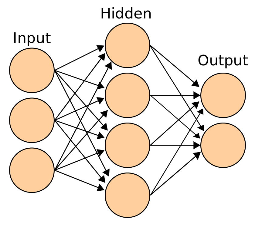
Figure 1: A graphical depiction of what a neural network looks like

On a smaller scale, each artificial neuron is connected to all of the following layer’s artificial neurons. A preceding layer’s neuronal output is the input, or x-values for the following layer’s artificial neurons. The strength and weight of this artificial neuronal connection is represented by a w-value which are tuned during the training process to better match the right inputs and outputs of the neural net. The transfer function in Figure 2 below represents the sum of the products of each input and its corresponding weight value. 

The weighted input is then fed into a non-linear activation function, which is a function that will convert the sum of weighted inputs into a number that the neuron can then output to the next layer. This function is very important because it allows neural networks to model a wider range of processes when compared to other machine learning methods. The produced number is often called the activation level and can represent how “strongly triggered” that neuron is by the input pattern. The strengthening or weakening of a neuron’s activation level can activate specific patterns of neurons in response to certain stimuli, resulting in neural network learning. 

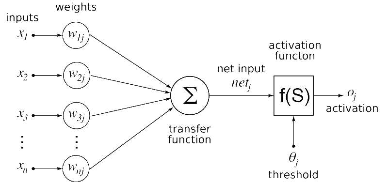
Figure 2: This is a model of a single node of a Neural Network. The inputs correspond to values fed in from each node in the prior layer. The weights correspond to a scalar constant that represents the “strength” of that node’s connection with the current node. The product of these weights and inputs are then summed up across all the nodes and connections from the prior layer and are then inputted into an activation function which will give the activation value for the current node.

Now that we have answered the question of how a neural network is represented, we can examine what learning really means in the context of a neural network. To better understand this, we can consider the common example of trying to build a handwritten number identifier, where the program’s goal is to correctly determine what digit (0 – 9) is written on a piece of paper. When presented with a handwritten 3, our untrained neural network is going to be fed a series of data points that represent how dark or bright a given pixel at a certain location of the image is. Our neural network will then process these inputs by multiplying the inputs with corresponding weight values, summing up the resulting values, and then applying the activation function to get the inputs for the next layer of neurons. These steps will result in some output corresponding to what the neural network “thinks” represents an appropriate outcome. 

At this point, a cost function comes into play. The cost function is a function that returns the difference between the expected output and the actual output for a set of data by assessing all the weights, or w-values. Ideally, our model would be perfect and our cost function would return zero every time. In order to get our model as close to ideal as possible by minimizing the cost function, the gradient descent enters the picture. 

At its simplest, gradient descent is a mathematical tool for finding the direction of steepest descent. In multivariable calculus, the gradient of a point on a surface represents the direction that has the steepest increase. For example, if you were standing somewhere on a mountain, the gradient from your perspective would correspond to the direction of steepest ascent. The gradient could be represented mathematically as a partial derivative of height over change in that direction. It is therefore also true that the negative gradient represents the direction of steepest descent. Gradient descent builds on these ideas by finding the direction of steepest decrease, “moving” in that direction, and then finding the direction of steepest decrease again by taking the negative of the gradient. This is kind of like a ball rolling down a hill. 

In the context of neural networks, negative gradient descent derivatives represent how the output will change with relation to each weight value by calculating the negative partial derivative of the output with relation to each w-value in the whole network. These weight values change according to the principles of gradient descent for each batch of training data that the neural network is trained on. Iteratively repeating the process of running the neural network on a set of training data points, applying a gradient descent protocol, and adjusting the weights of the network, allows the network to activate very specific neural patterns in response to specific inputs thereby allowing it to learn, minimizing its cost function. 

By representing learned trends via self-generated neural activity patterns, neural networks take a unique approach to the problem of developing learning algorithms, bringing mankind one step closer to developing computers and artificial intelligence systems that learn more like us. 

 

Sources:

(n.d.). Retrieved from https://www.google.com/search?tbs=sur:fc&tbm=isch&q=activated+neural+network&chips=q:activation+neural+network,g_1:machine+learning,online_chips:artificial+neural&usg=AI4_-kQiGc6V-SXjvFT1cocdn-mye4JyBQ&sa=X&ved=0ahUKEwjstueorr7lAhVBrZ4KHbXFBYAQ4lYIMSgE&biw=1229&bih=539&dpr=1.56#imgrc=ImBSCipO7xq0PM:

(n.d.). Retrieved from https://www.google.com/search?tbs=sur:fc&tbm=isch&q=activated+neural+network&chips=q:activation+neural+network,g_1:machine+learning,online_chips:artificial+neural&usg=AI4_-kQiGc6V-SXjvFT1cocdn-mye4JyBQ&sa=X&ved=0ahUKEwjstueorr7lAhVBrZ4KHbXFBYAQ4lYIMSgE&biw=1229&bih=539&dpr=1.56#imgrc=oZ0L7iwvPEG7HM:

(n.d.). Retrieved from https://www.youtube.com/watch?v=aircAruvnKk&list=PLZHQObOWTQDNU6R1_67000Dx_ZCJB-3pi&index=1.

(n.d.). Retrieved from https://www.youtube.com/watch?v=IHZwWFHWa-w&list=PLZHQObOWTQDNU6R1_67000Dx_ZCJB-3pi&index=2.

(n.d.). Retrieved from https://www.youtube.com/watch?v=Ilg3gGewQ5U&list=PLZHQObOWTQDNU6R1_67000Dx_ZCJB-3pi&index=3.

(n.d.). Retrieved from https://www.youtube.com/watch?v=tIeHLnjs5U8&list=PLZHQObOWTQDNU6R1_67000Dx_ZCJB-3pi&index=4.

Calculus on Computational Graphs: Backpropagation. (n.d.). Retrieved from http://colah.github.io/posts/2015-08-Backprop/.

File:Artificial neural network.svg. (n.d.). Retrieved from https://commons.wikimedia.org/wiki/File:Artificial_neural_network.svg.

Gradient. (2019, November 5). Retrieved from https://en.wikipedia.org/wiki/Gradient.

Neural Networks, Manifolds, and Topology. (n.d.). Retrieved from http://colah.github.io/posts/2014-03-NN-Manifolds-Topology/.